AI server power supply efficiency is not one fixed percentage. It is a curve shaped by accelerator workload, AC input, inlet temperature, airflow, module sharing, and the point where power is measured. A meaningful evaluation measures real AC input and DC output at the same operating point, repeats the measurement across representative workload states, and records redundant configurations separately. PSU conversion loss must also be distinguished from losses in the PDB, cables, UPS, and cooling system. Without those boundaries, two efficiency figures may describe different parts of the infrastructure and cannot be compared reliably.
Quick answer: measure a curve with a named boundary
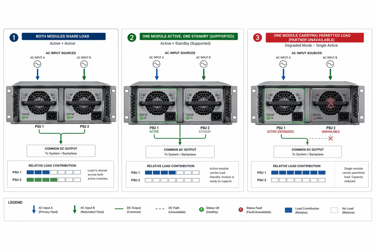
For each AI server operating state, record the PSU’s real AC input power, DC output power, input voltage, inlet temperature, airflow condition, active module count, and sharing policy. Calculate steady-state PSU efficiency as DC output divided by real AC input. For workload transitions, compare input and output energy over the same time window rather than dividing two unsynchronized instantaneous readings. Repeat the test for normal sharing, any supported standby policy, and the required degraded state. Keep downstream PDB and cable losses outside the PSU result unless the metric is explicitly defined as end-to-end server power-path efficiency.
One percentage can hide three different measurement boundaries
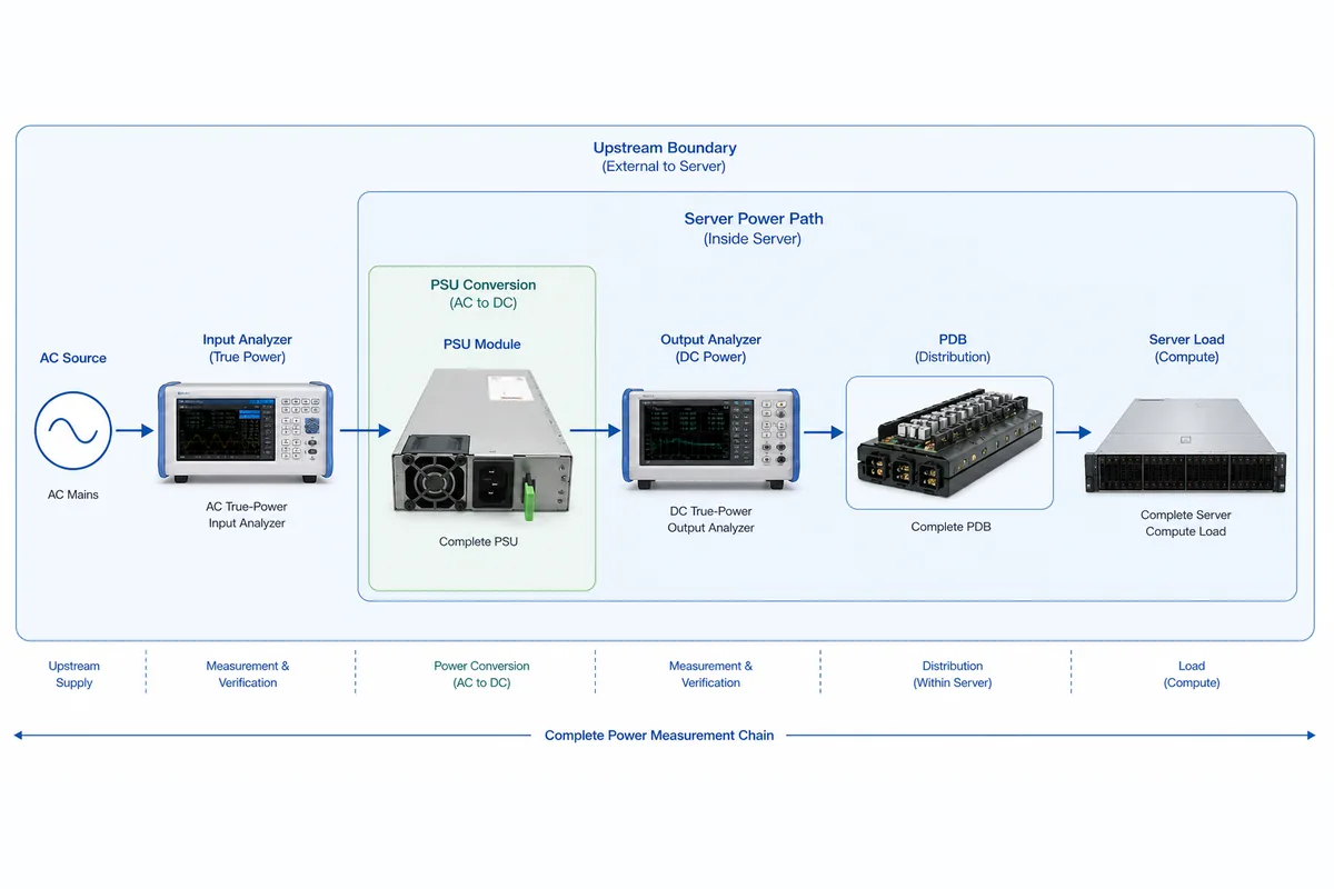
The word “efficiency” is often attached to measurements taken at different locations. The narrowest boundary covers the conversion module itself. A broader server boundary includes the PDB, connectors, busbars or cables, standby circuits, and potentially system fans. A facility metric can extend through the rack PDU, UPS, power distribution, and cooling plant. All are useful, but they answer different questions.
| Measurement boundary | Inputs and outputs | Question answered | Losses included |
|---|---|---|---|
| PSU conversion | Real AC power at the PSU input and DC power at its output interface | How efficiently does the PSU convert power at this operating point? | Internal switching, conduction, magnetic, control, and internally powered cooling losses |
| Server power path | AC entering the installed PSU set and DC delivered at defined server load points | How much power is lost before energy reaches the motherboard and accelerators? | PSUs plus the included PDB, isolation devices, connectors, cables, and distribution copper |
| Facility to useful load | Facility or UPS input and a defined server or computing output | What is the wider infrastructure cost of delivering power to the workload? | Upstream distribution, UPS, rack conversion, server distribution, and any cooling scope explicitly included |
For the PSU-only result, steady-state conversion efficiency is:
Efficiency (%) = DC output power ÷ real AC input power × 100
The AC instrument must report real power. Multiplying RMS voltage by RMS current produces apparent power unless power factor and waveform behavior are properly accounted for. On the DC side, the measurement must include every output rail inside the declared boundary. Measuring only the main output while omitting standby or auxiliary consumption can make the result appear better than the installed system actually performs.
Measurement location also determines whether distribution loss is visible. A DC reading at the PSU connector gives a module-level result. A second measurement near the accelerator or motherboard load shows how much is lost through the intervening path. In a redundant server, that path may include current-combining and fault-isolation elements described in the redundant power supply distribution board architecture. Those losses should not be silently attributed to the PSU, but they should not disappear from the server power budget either.
Build the curve from AI workload states, not two synthetic endpoints
A nameplate rating establishes a capacity boundary under documented conditions; it does not show where an AI server spends time or how efficiently the installed supplies operate there. Representative test points should come from the server’s actual workload profile. The objective is not to create one universal AI benchmark, but to expose the operating regions that matter for the intended deployment.
| Operating state | What to control | What the measurement reveals |
|---|---|---|
| Off or standby state | Installed modules, management state, auxiliary loads, and network accessibility | Baseline consumption that can be significant across a large idle fleet |
| Idle server | Boot state, accelerator power policy, fan policy, and background services | Part-load behavior when the converters may operate far below their rated output |
| Typical inference or mixed compute | Representative model, batch behavior, CPU participation, memory activity, and utilization | The efficiency region associated with normal production demand |
| Sustained accelerator load | Stable workload duration, cooling state, clocks, and any supported power limits | Conversion loss and thermal behavior near the deployment’s high-load region |
| Workload transition | Repeatable start time, sampling interval, synchronization, and observation window | How input energy and output delivery behave while demand changes rapidly |
| Required degraded state | Authorized module or feed condition, workload policy, and remaining cooling | The efficiency and loss concentration after power shifts to fewer active modules |
The workload must be documented with enough detail to reproduce its electrical behavior. “AI training” alone is not a test condition: model size, accelerator utilization, CPU and memory activity, communication traffic, cooling policy, and software power controls can all alter demand. For architecture context around accelerator branches and load movement, see Powernexu’s discussion of 2U GPU server redundant power.
Steady-state and transition measurements need different treatment
At a stable operating point, average real input and DC output over a defined period after temperatures and fan behavior have settled. Record whether the server was still thermally ramping; otherwise, a rising fan load may be mistaken for converter drift.
During a workload step, dividing one instantaneous output sample by one input sample can produce a misleading “efficiency” value. The PSU contains energy-storage elements, while input and output instruments may have different bandwidth, filtering, and timestamps. A more defensible transient metric compares energy entering and leaving the declared boundary over the same synchronized interval:
Windowed transition efficiency = DC output energy ÷ AC input energy
The interval should be long enough to include the relevant load transition and subsequent settling behavior, while still preserving the event the engineer intends to study. Retain the input-power, output-power, voltage, and workload traces rather than reporting only the calculated ratio. That evidence can show whether an unusual result came from genuine conversion behavior, stored energy, instrument timing, a power cap, or a cooling response.
Four conditions can move the curve after the workload is fixed
| Condition | Test record | Why it matters |
|---|---|---|
| AC input | Record voltage, frequency, source quality, and each module’s feed. | Current and conversion loss can change. |
| Inlet temperature and airflow | Measure PSU inlet temperature after stabilization; record airflow and fan policy. | Component and fan losses can change. |
| Redundant policy | Test supported sharing, standby, and degraded states separately; include every installed module’s input. | Each policy shifts module load. |
| Current sharing | Capture per-module input power and qualified telemetry. | Aggregate load can hide imbalance. |
Aggregate efficiency equals total declared DC output divided by total real AC input. Document telemetry calibration, filtering, update rate, and measurement location. Perform live-removal testing only when platform documentation, capacity, safety procedures, and continuity plans permit it; otherwise use qualified evidence or a controlled representative setup.
Read loss mechanisms without turning component technology into a guarantee
A high-power server PSU commonly contains power-factor-correction and isolated conversion stages, although the exact topology varies by design. Its total loss can include semiconductor conduction and switching loss, magnetic and capacitor loss, control power, current sensing, internal fans, and auxiliary rails. Part-load performance may be influenced by how stages enter or leave operating modes; high-load performance may be dominated by conduction, magnetic, and thermal constraints.
Wide-bandgap devices such as gallium nitride or silicon carbide can enable higher switching frequency, lower switching loss in suitable operating regions, or more compact magnetic components. They do not by themselves prove that a complete PSU is more efficient. Device selection, topology, gate drive, magnetics, layout, cooling, control strategy, input range, and workload point determine the result. Compare measured curves and documented conditions rather than inferring system efficiency from one semiconductor family.
An efficiency certification or standards-based test report can provide valuable evidence, but it must be read with its scope intact. The tested input, loading points, ambient condition, module configuration, and measurement boundary may differ from the deployed AI server. The ITU-T L.1241 methodology provides an authoritative framework for evaluating the functionality and performance of power supplies configured for servers. It does not remove the need to map the documented test conditions to the actual host, workload, and redundant policy.
Convert an efficiency difference into loss at the same DC output
Efficiency percentages become operationally meaningful when converted into heat and input energy at a common delivered load. Consider a hypothetical AI server requiring a steady 6 kW of DC output. The following values illustrate the calculation; they are not claimed specifications for a particular PSU.
- At an assumed 94% conversion efficiency, AC input is approximately 6 ÷ 0.94 = 6.383 kW, so PSU conversion loss is about 0.383 kW.
- At an assumed 96% conversion efficiency, AC input is 6 ÷ 0.96 = 6.250 kW, so PSU conversion loss is 0.250 kW.
- The difference is approximately 0.133 kW of electrical input and heat at that operating point.
If that exact load and efficiency difference persisted continuously for a year, the input-energy difference would be about 1.16 MWh. Real AI servers do not necessarily remain at one load continuously, so an annual estimate should integrate each workload state’s measured input power over its expected duration. Cooling energy, UPS loss, and downstream distribution loss remain outside this PSU-only example unless they are added through separately defined measurements.
This calculation also shows why percentage-point comparisons must use the same output power. Comparing two AC input readings while the workloads delivered different DC output does not isolate PSU efficiency. The workload, module policy, input condition, and thermal state must be aligned before the loss difference can be attributed to conversion performance.
A credible efficiency curve carries its evidence with it
A graph is useful only when another engineer can determine what each point represents. The supporting record should preserve the configuration and unresolved assumptions rather than presenting a smooth line detached from the server that produced it.
| Evidence field | Record for every curve or test series | Reason |
|---|---|---|
| Hardware identity | Server configuration, PSU model and revision, installed quantity, PDB, and relevant firmware | Prevents results from being transferred to a different assembly without evidence |
| Measurement boundary | Exact AC and DC measurement points, included rails, auxiliary loads, and excluded distribution stages | Defines what the efficiency percentage contains |
| Instrumentation | Instrument identity, calibration status, channel arrangement, bandwidth, sampling, and synchronization | Exposes uncertainty and transient-measurement limitations |
| Input condition | Measured voltage, frequency, feed assignment, and source condition | Connects the result to a deployable rack input |
| Workload state | Application state, utilization behavior, power policy, duration, and transition trigger | Makes the electrical operating point reproducible |
| Thermal condition | PSU inlet temperature, airflow or fan policy, stabilization time, and relevant chassis state | Separates conversion behavior from a changing cooling condition |
| Redundancy state | Active module count, sharing or standby policy, feed state, and per-module observations | Shows how the installed architecture positioned each converter on its curve |
| Source and revision | Controlled test record, manufacturer report, or applicable methodology with revision date | Keeps published and measured evidence traceable |
The finished curve should answer four questions without additional interpretation: where power was measured, what the AI server was doing, which modules were active, and under what input and thermal conditions the point was obtained. It can then support rack input estimates, heat calculations, redundancy-policy comparisons, and vendor-data reviews without being mistaken for a universal property of every AI server or every load state.
The most useful result is rarely the highest isolated percentage. It is a repeatable set of operating points that exposes where conversion loss occurs during the workload states the deployment will actually use. That curve shows whether an apparent advantage persists at part load, sustained accelerator demand, workload transitions, and the supported degraded configuration—and whether it belongs to the PSU itself or to a wider power path.