A high-efficiency industrial power supply should be specified by the losses it produces across the machine’s actual duty cycle, not by the highest efficiency percentage on a product page. Define the conversion boundary, identify how long the machine spends in standby, ready, production, peak, and other relevant states, and obtain efficiency evidence at the corresponding input, output, and thermal conditions. Convert each supported point into watts of loss and annual energy. This approach reveals whether an apparently efficient supply reduces enclosure heat and operating energy where the machine spends its time.
Quick answer: specify an efficiency envelope across the duty cycle
Replace “high-efficiency industrial power supply” in the purchasing specification with a table of operating states. For each state, state the expected DC output, input voltage, ambient or inlet temperature, cooling arrangement, annual operating time, and required efficiency evidence. Calculate conversion loss as output power multiplied by the quantity one divided by efficiency, minus one. Weight loss in watts by operating hours to estimate annual energy loss. Keep startup energy, wiring loss, downstream conversion, and undocumented conditions separate rather than hiding them inside one average percentage.
Put the efficiency boundary around the correct hardware
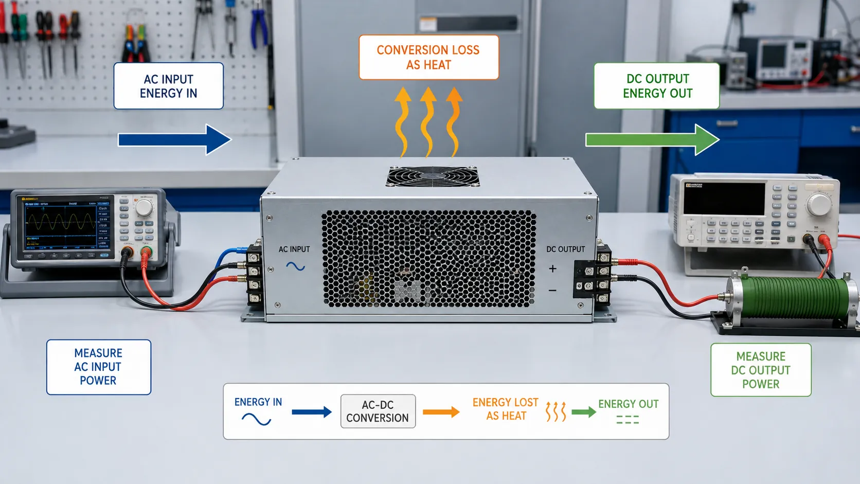
Efficiency is the ratio of useful output power to input power across a defined boundary. For an AC-DC supply, input power should normally be measured as real AC power at the supply input terminals or inlet. Output power is measured at the stated DC output terminals. For a multi-output unit, the relevant output is the sum of the power delivered by all outputs included in the test.
The basic relationship is:
Efficiency = total measured DC output power ÷ measured real input power
An efficiency value cannot be compared reliably until both measurement locations are known. One supplier may state efficiency for the converter alone, while a system measurement may include input filtering, output wiring, an ORing stage, distribution conductors, or auxiliary cooling. Both results may be useful, but they describe different boundaries.
| Boundary question | What must be defined | Reason it changes the result |
|---|---|---|
| Where is input measured? | At the PSU inlet, terminal block, upstream disconnect, or machine input | Upstream wiring, filters, and protection may add losses outside the converter |
| What counts as output? | Main output only, all regulated outputs, or power delivered at the load | Standby rails and downstream wiring can alter the reported ratio |
| Which auxiliaries are included? | Internal fan, external cabinet fan, control electronics, or remote modules | An externally powered cooling device is part of machine energy but may be outside PSU efficiency |
| What product is being evaluated? | Enclosed supply, open-frame board, encapsulated module, or configurable system | Different packages leave different integration and cooling functions to the machine |
If shortlisted products do not represent the same physical and conversion scope, first normalize them using the industrial AC-DC power supply module classification framework. Classification should remain a short preliminary step here; the loss budget begins only after every candidate has a stable measurement boundary.
Power factor and efficiency also answer different questions. For AC input, apparent power and input current affect conductors and upstream equipment, while efficiency connects real input power to delivered DC power. A true-power measurement is therefore needed for the efficiency calculation; multiplying nominal voltage by current without accounting for waveform and power factor may not provide the required real-power value.
The machine duty cycle determines which efficiency points matter
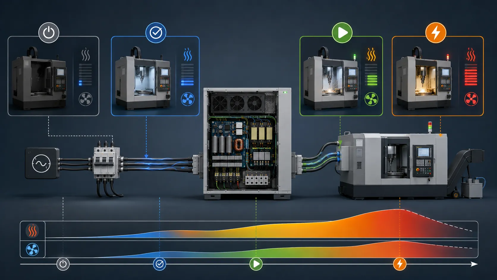
Define only recurring or decision-relevant states: standby, ready or idle, normal production, peak production, and any supported degraded mode. For each state, record DC output, annual hours or an hours range, input condition, ambient or inlet temperature, cooling arrangement, and the nearest model-specific efficiency evidence. The longest-running state can dominate annual loss even when it is not the highest-power state.
Treat startup and recovery separately when voltage and current change too quickly for a steady-state efficiency value. Use documented inrush, transient, sequencing, or energy-per-start data where needed. Do not invent a steady-state efficiency point for a transition, and do not add states that have no material effect on selection or annual loss.
Convert supported efficiency points into loss and heat
At each documented operating point, calculate:
Input power = output power ÷ efficiency
Conversion loss = output power × (1 ÷ efficiency − 1)
Annual conversion loss = loss watts × operating hours ÷ 1,000
The following assumed values illustrate the weighting method; they are not specifications for any product.
| State | Hours | DC output | Efficiency | Loss | Annual loss |
|---|---|---|---|---|---|
| Standby | 1,760 | 15 W | 55% | 12.3 W | 21.6 kWh |
| Ready | 2,000 | 80 W | 85% | 14.1 W | 28.2 kWh |
| Normal production | 4,500 | 400 W | 93% | 30.1 W | 135.5 kWh |
| Peak production | 500 | 700 W | 94% | 44.7 W | 22.3 kWh |
These rows produce approximately 207.6 kWh of annual conversion loss. The aggregate efficiency is total DC energy divided by total AC input energy—about 91.8% here—not the arithmetic mean of the four percentages. Normal production dominates annual loss, while peak production creates the greatest instantaneous heat. Conversion loss ultimately becomes heat, but component temperatures still depend on airflow, orientation, thermal resistance, and neighboring heat sources.
Do not extend a documented point beyond its conditions
A peak efficiency figure may be valid yet irrelevant to the intended machine. Each point in the loss budget needs evidence that covers, or credibly bounds, the associated line, load, and thermal condition. The supplier’s technical material should indicate enough of the following coordinates to make the value interpretable:
- exact manufacturer model and applicable revision;
- nominal and actual input voltage and frequency for AC-DC equipment;
- DC output voltage, current, and treatment of secondary or standby outputs;
- load percentage or measured output power;
- ambient or inlet temperature and stabilization condition;
- cooling method, airflow direction, flow assumption, and orientation where relevant;
- measurement boundary, instrumentation method, and applicable tolerances;
- derating or operating restrictions affecting the stated point.
Input voltage matters because conduction, switching, magnetics, and control losses do not remain in identical proportions across the complete line range. A universal-input rating establishes an allowed operating range when supported by the model documentation; it does not establish one efficiency value throughout that range.
Temperature and cooling require similar care. An efficiency value measured under a controlled laboratory condition does not automatically describe a sealed control cabinet near the upper end of the supply’s permitted ambient range. Derating can also make a candidate unsuitable even when its efficiency remains attractive: if the supply cannot deliver the required output under the installed thermal condition, the efficiency number does not rescue the design.
The interaction between industrial AC-DC efficiency, thermal stress, topology, and reliability is discussed in this Texas Instruments technical article on industrial power-supply efficiency and reliability. Component or topology choices can influence achievable performance, but they should not be treated as a guarantee of system efficiency without model-specific operating evidence.
Parallel or redundant industrial supplies introduce another condition. Sharing a load across two modules can move each converter to a different point on its efficiency characteristic. A supported module-shedding policy may improve part-load operation in some architectures, while a required always-on redundant configuration can prioritize availability. Compare the actual supported operating modes rather than applying the single-module peak value to the complete system.
Make the loss budget enforceable in the RFQ
A purchasing requirement needs more than a request for an efficiency curve. It should connect each required point to the quoted model and identify what happens when evidence is missing. A compact schedule can request:
- The exact product identity, revision control, package type, input and output configuration, and supplied accessories.
- An efficiency table or traceable input/output data at the specified line, load, temperature, and cooling conditions.
- Maximum or guaranteed values where the loss budget is a contractual limit, rather than typical values presented only for reference.
- Derating, standby consumption, internal-fan consumption, output-cable boundary, and secondary-output treatment.
- A declared tolerance or acceptance band accounting for product variation and the agreed measurement method.
- Identification of duty-cycle rows that remain unsupported, require interpolation, or need application testing.
Do not silently fill an undocumented load point by drawing a smooth line between two catalog values. Interpolation may be useful for preliminary modeling when the supplier agrees that the method is reasonable, but the estimate should remain identified as an estimate. Extrapolation beyond documented load, line, or temperature conditions is more uncertain and should not become a guaranteed requirement without supporting evidence.
Example requirement language: The quoted power supply shall include model-specific efficiency or measured input/output evidence for the operating points in the attached duty-cycle schedule. Every value shall identify the input, output, thermal, cooling, and measurement conditions. Unsupported points shall be marked unresolved rather than represented by a family-level peak efficiency claim.
For a rack-based industrial system, the PSU loss budget may be only one part of a wider source, distribution, cooling, and service definition. The industrial rackmount power supply RFQ framework shows where these wider subsystem responsibilities belong without merging them into the converter-efficiency figure.
Acceptance measurements must reproduce the specified boundary
Incoming inspection can confirm identity and documentation, but an efficiency acceptance measurement requires a controlled electrical setup. The test plan should use the same measurement boundary and operating coordinates that created the requirement.
For AC-DC equipment, measure real input power with equipment suitable for the waveform and expected power range. Measure output voltage and current at the agreed terminals, including every output counted as useful power. Allow the supply and test load to reach the specified stable thermal condition. Record input voltage, frequency, output load, ambient or inlet temperature, orientation, airflow, auxiliary consumption, and instrument uncertainty alongside the result.
A single reading at room temperature and nominal line cannot accept requirements written for multiple line and thermal conditions. Conversely, production acceptance does not necessarily need to repeat every engineering characterization point. The contract can distinguish among supplier design evidence, initial sample evaluation, periodic verification, and production screening. The required scope depends on the consequence of missing the loss budget and the confidence supplied by the model-specific documentation.
Measurement uncertainty should be considered before setting a pass/fail threshold. If the required difference between two candidates is smaller than the combined uncertainty and expected unit variation, a measured ranking may not be reproducible. Procurement language should also distinguish typical performance from a guaranteed minimum efficiency or maximum loss. These are different commercial commitments even when the nominal percentages appear identical.
The most efficient catalog point may not produce the lowest-energy machine
A candidate with the highest peak percentage can lose the duty-cycle comparison for several reasons. It may spend most operating hours far below the load where its peak occurs, require an auxiliary fan that is outside the published efficiency boundary, or lack evidence at the machine’s actual input and cabinet temperature. An oversized supply can also operate at a lower load fraction for much of its life. Oversizing may still be justified by startup demand, output transients, derating, expansion, or reliability objectives, but the energy consequence should be visible.
Architecture can outweigh small converter differences. Eliminating an unnecessary conversion stage, reducing excessive distribution loss, or using a supported low-power state can save more energy than selecting between two supplies with nearly identical documented efficiency near full production load. Those changes require separate analysis because they can alter isolation, hold-up behavior, protection coordination, controls, and machine availability.
The duty-cycle loss budget keeps these choices comparable without declaring one universal winner. It identifies the instantaneous heat produced in each supported state, the annual energy associated with credible operating hours, and the rows where evidence is still absent. “High efficiency” then becomes an enforceable property of an exact industrial power supply in a defined machine—not a free-floating adjective attached to its best catalog percentage.