Two suppliers can quote a high-voltage DC-input CRPS server power supply for the same host and DC voltage range, yet provide very different evidence about how it will behave on the rack feeder. The useful comparison begins after the modules have started and the servers are running. If the shared DC bus is briefly disturbed, do voltage and current settle while the same modules continue regulating? A supplier’s input-voltage range establishes one prerequisite. The answer about settling belongs to the connected source, feeder, filters, and active modules.
Quick Answer
Compare the source output impedance with the combined CRPS input impedance at the same electrical boundary and operating point. Multiple active modules can lower the combined input impedance when they add load to the feeder. Splitting an unchanged load can leave the low-frequency result unchanged under a constant-power approximation. Ask for evidence that covers the installed branches and relevant module states, with any protection intervention identified separately from ordinary settling.
Choose the electrical boundary before comparing impedances
Start at the rack distribution point where the DC feeder divides. Looking upstream from that point, the source output impedance describes how the plant and the common feeder respond to a small change in current. Looking downstream, the combined input impedance describes how the connected branches and their converters respond to a small change in voltage. Both quantities are measured or modeled across the same supply and return pair. A source curve measured at the rectifier cabinet and a module curve measured at its inlet describe different interfaces until the intervening network is accounted for.
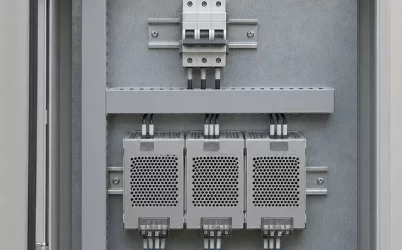
In the example rack, one enclosed DC distribution assembly serves two server chassis. Each chassis has its own branch run from that assembly. The branch runs and the shared feeder occupy different parts of the electrical model. A voltage disturbance developed on the common feeder can reach both branches, while a filter or cable on one branch can make the voltage at that module’s inlet differ from the voltage at the split.
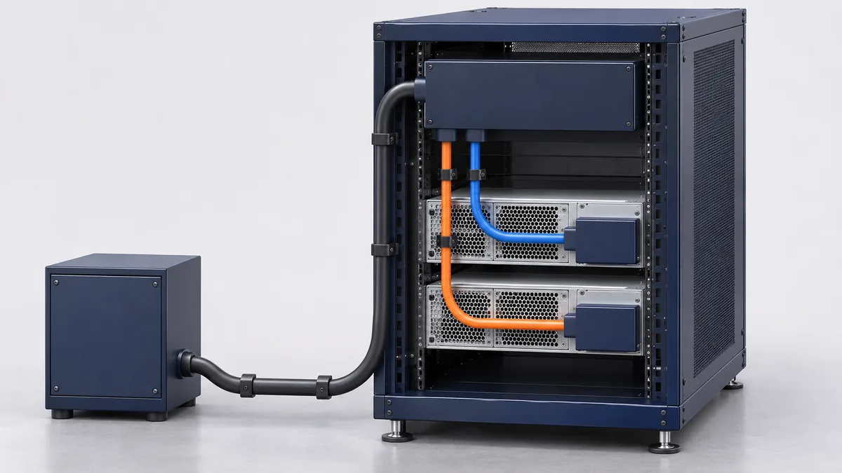
Assign each external filter to one side of the chosen boundary. A common filter ahead of the split belongs in the upstream impedance when the comparison is made at the split. A branch filter beyond that point belongs in the downstream network. If the module’s measured input impedance already includes its internal filter, that measurement represents the complete module at its terminals. Adding a second model of the same filter would change the predicted resonance. Moving the comparison point is valid if both sides are recalculated at the new point.
At a common pair of nodes, the same small voltage perturbation appears across every parallel branch, and the branch current perturbations add. That is why branch admittances, the reciprocals of their complex impedances, can be summed at that pair. Each admittance must represent the whole branch as seen from the common point. For a simple series branch lead, include its impedance before taking the reciprocal. A branch with shunt elements or a more elaborate filter needs its own network calculation or measurement. If modules also interact through shared output controls or other paths, characterize the connected group in its intended state. An independent module admittance measured with those paths absent can miss a coupled mode.
A NASA technical memorandum on distributed DC power systems applies this interface method to switching converters. It shows how parallel loads can bring the aggregate input impedance into the range of the source impedance and explains why magnitude overlap calls for further analysis. Its application is spacecraft power. The transferable part for a server rack is the source and load analysis at a defined interface. NASA Technical Memorandum 107281 on DC power-system stability.
Find the frequency band where the feeder matters
A regulated converter can draw more input current when its terminal voltage falls. Suppose the server load stays essentially unchanged and the converter draws approximately constant input power over the small variation and frequency band being examined. From I = P/V, the local slope of input current against voltage is approximately −P/V². The reciprocal, −V²/P, is the incremental input resistance in that approximation. The negative sign describes the direction of the response around an operating point. The module still draws positive average power from the feed.
That slope helps explain how an otherwise modest disturbance can persist. Cable inductance and input capacitance can exchange energy and produce ringing. Resistance and other damping mechanisms dissipate some of that energy. When the regulated input responds to a falling voltage by drawing more current, its incremental behavior can reduce the effective damping of the combined network. The result depends on the frequency of the resonance and how the source and load respond there. A low measured DC resistance through the feeder can coexist with a much larger source impedance near a resonance.
The constant-power approximation is tied to the operating point and to frequencies over which the actual input behaves that way. The converter’s regulation, input energy storage, filtering, and any change of operating mode can alter both the magnitude and phase of its response. Input capacitance may dominate in a band where the simple slope is unrepresentative. An operating point near a mode transition can also be a poor candidate for a single linear model. Keep the approximation attached to the conditions that justify it.
A conservative small-signal screen for stable source and load subsystems in a suitable single-interface model is to keep the source impedance magnitude below the load impedance magnitude across the relevant spectrum. The amount of separation required for acceptable performance is a project decision. Where the curves approach or cross, examine the complex ratio of source to load impedance, including phase and the assumptions about subsystem stability. A Nyquist assessment accounts for how that ratio approaches the critical point and for any open-loop unstable poles. Two magnitudes alone leave that judgment open. A favorable comparison over a narrow frequency sweep also leaves any unexamined modes outside its scope.
Hold total power fixed, then hold per-module power fixed
Consider a hypothetical rack with a settled voltage of 300 V across the common input pair. Compare one active module with two active modules under two different workload assumptions. For the calculation, both branch impedances are negligible over the band of interest, the modules respond independently, and the inputs behave as constant-power loads across that band. All power figures refer to the DC input of the modules. They are invented operating points for the example.
| Active configuration | Total input power | Combined incremental input resistance |
|---|---|---|
| One module at 900 W | 900 W | −100 Ω |
| Two modules at 450 W each | 900 W | −100 Ω |
| Two modules at 900 W each | 1,800 W | −50 Ω |
In the first case, 300² divided by 900 gives a magnitude of 100 Ω. In the second, each module contributes an incremental resistance of −200 Ω. The two admittances add to give an equivalent resistance of −100 Ω. Adding a second active module while holding total input power fixed therefore leaves the calculated slope at the common node unchanged. In the third case, each module contributes −100 Ω, so the combined resistance is −50 Ω. The same small voltage change now produces twice the total change in input current predicted for the 900 W cases.
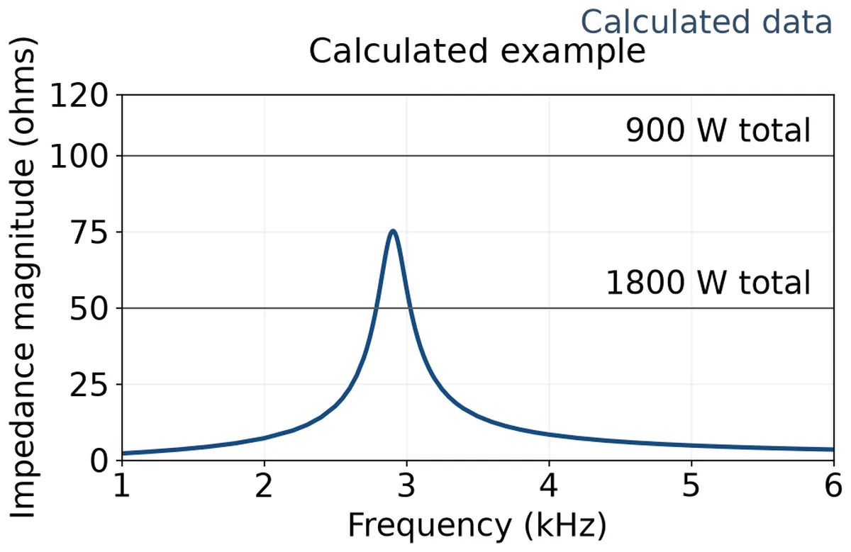
Give the example feeder a frequency-dependent output impedance. Model the upstream supply as an ideal voltage source behind 0.40 Ω of effective loop resistance and 300 µH of loop inductance, with a 10 µF shunt capacitor across the common pair on the source side of the comparison boundary. The 300 V operating point is stipulated for each case. The ideal supply’s DC setting can differ between cases to account for the changed drop across the series resistance. Its small-signal impedance model is the same in all three.
With the ideal source set to zero for the small-signal impedance calculation, the series resistance and inductance are in parallel with the shunt capacitor. The resulting source impedance magnitude peaks at about 75 Ω near 2.9 kHz. In the two 900 W total-load cases the assumed load magnitude is 100 Ω, so the source stays below it in the plotted band. At 1,800 W the load magnitude falls to 50 Ω and the curves overlap near the peak. The plot shows where the magnitude screen calls for phase information. The modeled values describe a hypothetical network and carry no equipment rating or deployment verdict.
The two comparisons answer different engineering questions. If an additional server brings its own workload onto the same feed, holding the original per-module demand fixed captures the increased aggregate power in this example. If the host redistributes the same workload among more active supplies, start with total input demand at the feeder and find the operating point of each module. Even when total input power happens to stay fixed, a different control mode, connected input capacitance, or unequal branch impedance can change the response outside the constant-power approximation. A connected module whose main output is idle may still contribute input admittance. Count it according to its electrical state and the applicable evidence.
Read the decay before the system changes state
A useful disturbance record shows an initial settled operating point, a bounded excitation, and the response after that excitation has ended. If the test uses a small pulse, compare successive peaks about the same baseline after the pulse. If it uses a small step, judge settling around the new steady level. A diminishing envelope while the source and all intended modules continue regulating supports damping of the modes excited and observed in that configuration. A flat tail alone says little if the record ends too soon to reveal a slower oscillation.
A growing envelope after the stimulus ends warrants investigation of the energized network. Sustained ringing also calls for a look at the stimulus and the rest of the system. A periodic workload or source ripple can keep exciting a damped resonance. The time trace can show persistence without identifying its cause. Compare the drive and response on a common time base, and retain the source and module states through the interval of interest. If the excitation was too small for the response to rise above noise, a flat record provides weak evidence about damping.
Suppose an example trace shows several oscillations before one module stops drawing its previous branch current and the bus becomes quiet. If synchronized status and current evidence shows that the module entered protection, the quiet tail describes a different population or control state. It gives no decay result for the original state. The same distinction applies if the upstream source enters current limit or the host reduces load. A successful protective response may be valuable for a fault requirement. For a small-signal comparison, evaluate the interval during which the original operating state still holds.
Ask for the shared-bus voltage and, where the branch network matters, voltage at the affected module inlet. Pair those traces with common feeder current, relevant branch currents, and available source or module status. Oscillation on one branch may be less visible at the common point, especially if branch current variations partially cancel. A coarse management log can provide context about a state change. Its update rate and timing determine how closely it can locate that change relative to the electrical waveform. Energized HVDC characterization belongs with qualified personnel using the platform’s approved test arrangement and appropriately rated instrumentation.
Compare supplier reports against the same energized rack
For an impedance-based submission, request the measured or modeled frequency range, magnitude and phase, exact port, and operating conditions. Ask which module revision and configuration the data represent, what output load each unit carries, and which other modules remain connected. The source configuration should identify the distribution path and any filter whose behavior is included. A report from a single module can supply a branch model when the recorded conditions match the branch’s intended operation and the assumptions about independent response are justified.
A time-domain submission can answer the same purchasing question by showing that an installed or electrically representative rack settles after an appropriate disturbance. The report should identify where and how the excitation was applied, its size and duration, which inputs and outputs were observed, and whether the system stayed in the stated control mode. A short disturbance and a slow ramp cover different frequency content. Before comparing two traces, establish that the stimuli excite the region of interest and that the observation windows capture the response long enough to assess it.
Where reports use different test fixtures, look for a defensible relationship between the fixture and the intended installation. A programmable source and short cable can characterize a module under a documented condition. A rack with a remote rectifier, longer loop, and external filter may present a different impedance near resonance. Conversely, an electrically representative fixture can be useful even when it is physically smaller than the rack. The relevant match is the impedance and connected behavior at the chosen interface under the required conditions.
Compare the operating cases the rack will actually use. A full-load report may cover a high aggregate demand while leaving a lightly loaded control mode or another rectifier configuration open. A supported reduced-population state can change the surviving modules’ operating points and leave powered but idle branches attached. If the rack uses both a normal plant configuration and another sustained source configuration, compare the evidence for each settled state. Source-transfer continuity requires its own assessment of the transition.
Consider two hypothetical bids. One supplies a clean response for the intended module population but uses a fixture whose impedance near the installed filter resonance is undocumented. The other supplies complex input data for the offered revision, and the rack engineer has matching source data, including that resonance. The second submission gives the engineer a way to assess interaction at the proposed interface, subject to the model and operating conditions. If that calculation exposes a lightly damped mode, an applicable system response becomes particularly valuable. The first submission can address the same gap by establishing electrical equivalence of its fixture or extending the result to a representative feeder.
The evidence can also identify which design owner has room to act. A source-side resonance common to several eligible loads points toward the distribution or filter design. A response that appears only when one candidate enters a specific regulation mode gives the module supplier a narrower question. A proposed damping change must be evaluated with the applicable equipment limits and other functions of the filter. If the rack layout or filter is already fixed, evidence for that exact feed is a stronger basis for the sourcing decision than a general promise that the candidate operates on HVDC.
Frequently Asked Questions
Can a short, heavy feeder rule out input resonance?
It can reduce part of the loop impedance. The complete source output impedance can still reflect rectifier controls, a shared filter, and other connections upstream of the split. If the installed arrangement changes a part of the network that contributed to the original impedance result, establish its response in the affected frequency band.
Can I use an input-impedance curve taken on AC for an HVDC installation?
Use evidence for the DC input mode of the offered revision. Even where the same module accepts both sources, its internal operating state and input-current response may differ. A supplier can establish applicability by explaining the relationship between the modes and providing supporting evidence for the frequency band and load of interest.
Does a matching resonance frequency make two suppliers’ results equivalent?
The frequency identifies where the response occurs. Compare the peak magnitude, damping, phase where available, and the operating states that produced it. Two systems can ring at similar frequencies and differ substantially in how long the disturbance lasts or how close it comes to an operating limit.
Can adding a capacitor at the rack improve stability?
Capacitance changes the impedance seen by the modules and can move or reshape a resonance. Its placement, losses, and interaction with the source and branch filters determine the effect. Evaluate any proposed capacitance or damping network against the actual response and the equipment’s permitted input network, including charging and protection requirements.