A server power supply MTBF figure estimates a population’s failure behavior under stated assumptions; it is not the number of hours a particular module is expected to last before replacement. An advertised 200,000-hour MTBF does not promise 22-plus years of service to one server. Its practical use is to estimate the frequency of random failures across many units during a defined operating period, then compare options only when their calculation methods and conditions are compatible.
The acronym means mean time between failures, although product literature sometimes uses it loosely for a nonrepairable module where mean time to failure would be the stricter term. That terminology matters less than the underlying model: what counts as a failure, whether the number was calculated or observed, what temperature and load were assumed, and whether the estimate applies only to the relatively steady random-failure phase. Without those details, a larger MTBF number is not necessarily stronger evidence.
Why 200,000 hours is not a replacement interval
MTBF is commonly derived from a failure rate, often represented by λ. Under a constant failure-rate assumption, MTBF is approximately 1/λ. The model describes a group of devices exposed to the same specified conditions. It does not say that every unit operates normally until an MTBF clock expires and then fails. Random failures are spread through time: some occur early, some much later, and many units can outlive the quoted interval.
For a constant hazard model, the chance that a unit has not failed by time t is R(t) = exp(−t/MTBF). At t equal to the MTBF, R is about 36.8%. This surprises readers who interpret the rating as a median or guaranteed operating life. The equation itself is conditional: it represents random failures within the model’s applicable interval, not the full aging behavior from first use through wear-out. It cannot tell when a particular power supply will fail.
A COSEL technical explanation of MTBF explicitly connects MTBF to the constant-failure-rate portion of the reliability curve and describes a part-count prediction method for its supplies. That is a useful illustration of why a specification number should be accompanied by its model and assumptions. Another manufacturer’s number may use a different method, environment or part set; comparing the two as bare hours can be misleading.
The distinction from service life is crucial. A module can reach a period in which fans, capacitors or other parts wear out and its failure rate is no longer roughly constant. MTBF calculations based on the earlier random-failure period do not grant an indefinite extension through that later phase. For deciding when to refresh a server fleet, the actual thermal history, observed faults, spare availability and vendor support matter alongside—but separately from—the MTBF figure.
What the calculation method has to disclose
Some MTBF values are predictions assembled from component failure rates using an established method. Others are based on test or field data, perhaps accelerated or limited in scope. A part-count prediction is not inherently dishonest; it is a model that needs a defined temperature, environment and component population. A field estimate is not automatically superior if the observation period, duty or failure definition is unclear. To interpret either, ask what was counted and under what operating conditions.
The failure definition can change the result. Is a PSU considered failed only if it stops producing output? Does a fan fault that leaves output temporarily available count? What about a telemetry fault, out-of-range voltage, nuisance shutdown or a unit removed for a suspect alarm? In a server, an unavailable module may degrade redundancy even if the load stays powered. A fleet operator may care about the loss of protected capacity before complete electrical failure. A supplier’s MTBF number may or may not use that same endpoint.
Temperature is another input, not a footnote. Semiconductor, capacitor and fan stresses respond differently to heat, and a rack inlet value may not equal the PSU component temperature. A calculated MTBF at one ambient should not be carried unchanged into a warmer or more obstructed chassis. Similarly, a high-line and a low-line operating point can impose different currents and losses. The data sheet or reliability report should say enough about test or prediction conditions to determine whether the number is relevant to the intended host.
Methods and standards can also differ in their treatment of component types, operating stresses and quality factors. A catalog page that prints only “MTBF: 200,000 hours” is incomplete as a basis for ranking unlike products. If a purchasing team requests reliability evidence, the useful comparison is not simply which number is larger; it is whether the same endpoint, method, environment and useful-life period were used. Where those cannot be aligned, the figures can still be reported but should not be scored as a clean numerical contest.
Manufacturing quality and screening belong in a separate part of the story. A model may have a low predicted random-failure rate yet experience early field failures if production defects escape screening. Another fleet can suffer failures caused by a shared installation error rather than the intrinsic converter design. MTBF arithmetic built from component tables cannot identify either pattern. Field-return classification and a consistent definition of exposed operating hours are necessary before a site uses its own observed incidents to challenge or refine a supplier prediction.
A hypothetical fleet calculation, with its limits visible
Suppose a hypothetical server PSU population has a constant-rate MTBF of 200,000 hours under conditions that genuinely match an installation. In one year of continuous operation, each module accumulates 8,760 hours. The model gives one module a no-failure probability of exp(−8760/200000), or roughly 95.7%. That does not mean the PSU “lasts 95.7% of a year.” It means the model predicts roughly a 4.3% chance of at least one random failure for a single unit over that particular year, assuming the model is valid throughout it.
For 100 independent, identically exposed modules, the expected number of random failures over that year is 100 × 8,760 / 200,000 = 4.38. An expected count is an average across many repetitions of the same scenario, not a promise that exactly four or five PSUs will fail. A real fleet may see fewer, more, or a cluster related to a shared cause. Statistical uncertainty becomes especially important when the input MTBF is itself a prediction rather than a well-supported field estimate.

The model can help size spare stock or service response at fleet scale, but it does not determine the spare inventory by itself. Sites differ in delivery time, repair policy and downtime cost. The modules may not be independent if they share a hot rack, a problematic feed, the same production lot or a common fan-control issue. A simple count also does not establish whether the server stays available when one PSU fails. That depends on the redundancy topology, surviving-module capacity, PDB isolation and workload behavior.
Now change only the assumption: imagine those 100 supplies enter a wear-out phase in which failure rate rises with age. The constant-rate arithmetic above would no longer describe the later period accurately. The formula cannot be made valid by merely plugging in more hours. The operating population and failure data need a model appropriate to aging, or the analysis should stop at the boundary of the available evidence.
Two PSUs do not automatically square the risk
A common shortcut treats two independent PSU failure probabilities as if their simultaneous loss were simply the product of the two probabilities. That can be a useful idealized calculation for a strictly defined interval and truly independent module failures, but it is not automatically the server’s availability. Both modules can depend on the same PDB, input feed, chassis cooling, firmware policy or service procedure. A common-cause event can remove both paths without violating either module’s individual MTBF specification.
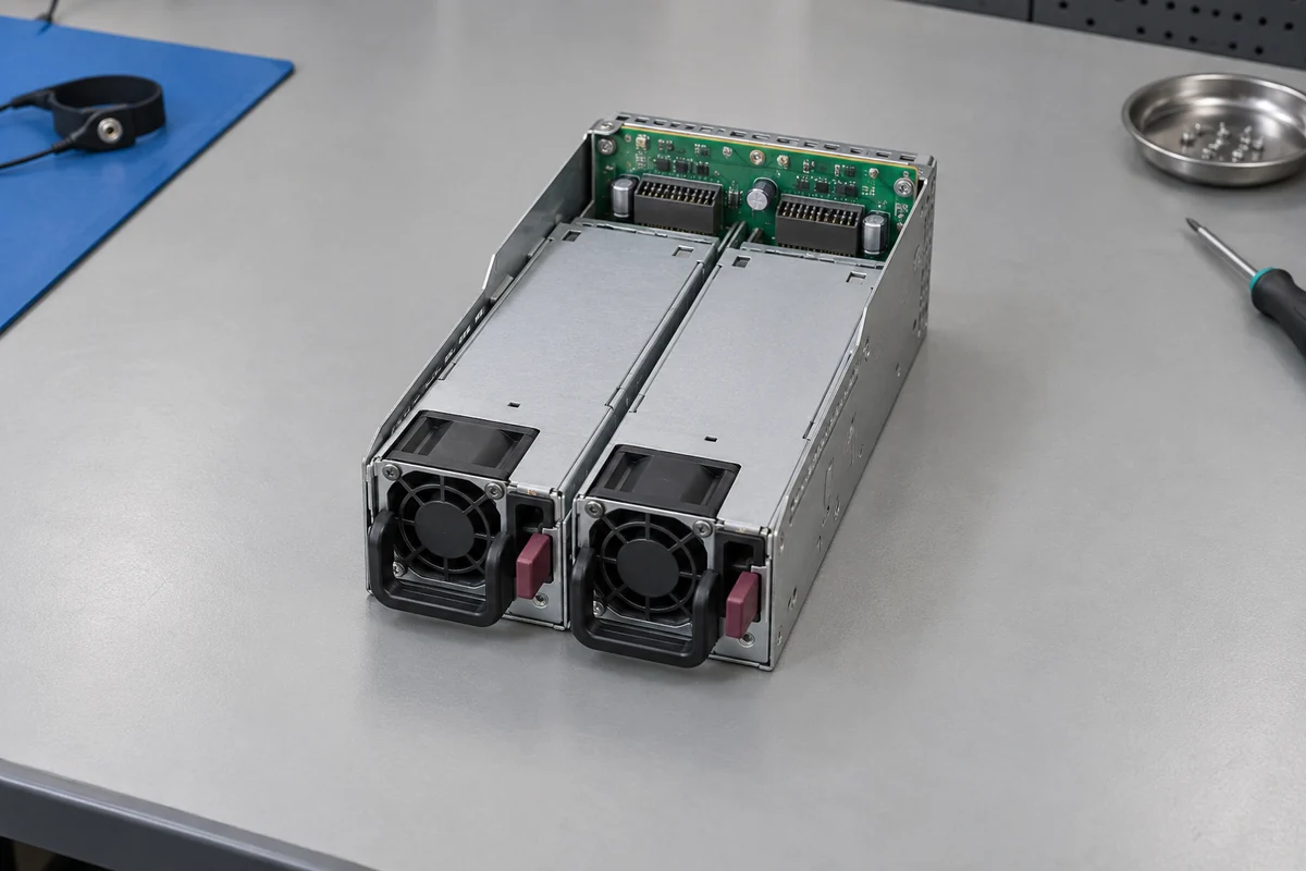
Redundant pairs can also spend unequal time under load. A current-sharing system may distribute output between modules; another arrangement may park one module in a low-power state. After a failure, the survivor’s current and temperature change. If the published MTBF applies to a different duty point, using the same figure for every state is unjustified. Module MTBF describes a population under specified conditions, not the complete 1+1 behavior during faults and maintenance.
A more precise reliability model would define failure states and restoration: one module lost but server running, second module lost before replacement, common feed lost, PDB fault, and repair time. Those state transitions have different impacts on protected service. The basic MTBF number may support one input to that model, but it cannot supply the whole model. A particularly high PSU MTBF does not compensate for a single unprotected distribution component or a repair process that leaves the system exposed for weeks.
The distinction between reliability and availability is useful here. Reliability asks whether a component operates without failure for an interval; availability accounts for both failure and restoration over time. A hot-swap spare and fast response can improve availability without changing the intrinsic MTBF of the PSU module. Conversely, poor fault detection or an unavailable replacement can magnify the service effect of a failure even if the module’s predicted MTBF is high.
What to compare when two quotations show different MTBFs
First identify the exact unit or assembly to which each figure belongs. A bare module, fan-inclusive assembly, power shelf and complete server are different objects. Then identify failure criteria and whether the figures are predicted or based on test or field evidence. Compare their stated ambient, load, input and cooling conditions. If one quote uses a 25 °C prediction for a component set and the other a 40 °C estimate for a complete fan-equipped supply, their hour counts do not form a fair ranking.
Where the method is disclosed, compare like with like. A predicted part-count value and a demonstrated value can both inform a discussion, but they answer different questions. Ask whether fans, connectors and electrolytic capacitors are included; whether wear-out is excluded; and what confidence or sample size accompanies a demonstrated result. This is not a demand that every product offer a complete reliability paper. It is a way to prevent a prominent number from silently standing in for evidence it does not contain.
For a server operator, the practical outcome may be to keep both values in a specification sheet while weighting other evidence more heavily: approved host compatibility, thermal limits at the actual inlet, fault telemetry, replaceability, warranty terms and observed fleet behavior. If one candidate has a much larger MTBF but cannot be used in the target chassis or loses output at the site’s input condition, the reliability number cannot rescue it. The specification must first describe the intended installation.
The number’s proper boundary
MTBF can be an engineering input for population-level random-failure planning when its assumptions are disclosed and applicable. It is not a countdown timer on an individual PSU, not a replacement schedule, and not a stand-alone measure of server uptime. Read the hours together with the calculation method, operating conditions, failure definition and useful-life boundary. Then use the figure for the question it can answer: a conditional estimate of failure frequency among comparable modules, not a guarantee about a particular machine.