
On an isolated AC-DC flyback schematic, the output capacitor sits on one side of the transformer and the switching controller sits on the other. If the DC output falls when a load draws more current, how does the controller know to respond? Start by finding the two points the regulator senses. They reveal whether the circuit measures the output itself or estimates it from the primary, and why connecting the secondary to earth need not change what the regulator sees.
How does feedback cross the isolation barrier?
In an isolated AC-DC flyback, the transformer transfers energy between separate windings. An optocoupler can send the secondary voltage error back as light. A primary-side regulator estimates the output from a reflected flyback voltage. A permitted secondary-to-earth bond sets the output’s earth reference while leaving the supply’s internal insulation barrier intact. Galvanic separation in the installed system also depends on conductive paths outside the supply.
The transformer carries energy to the output
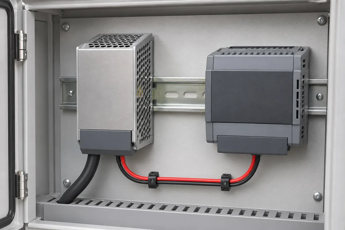
Consider an industrial AC-DC supply feeding a separate controller inside a metal enclosure. The mains conductors end at the supply, and two DC conductors continue to the load. That physical arrangement helps locate the two power interfaces, but the closed supply hides both its insulation boundary and its sensing circuit. To find either one, turn to the circuit drawing. In this example, the supply contains a single-output flyback with a diode rectifier, and the load has its own DC return conductor.
Inside the supply, the input rectifier and bulk capacitor create a DC bus for the primary switch. The negative side of that bus is the primary controller’s local reference. A schematic may mark it with a ground symbol, but it is still part of the mains-connected circuit. The secondary return is the reference for the output filter and load. The transformer has separate windings, so neither side needs to borrow the other side’s return conductor to transfer energy.
Texas Instruments’ archived application note Isolated Supply Overview and Design Trade-Offs describes the two switching intervals. While the primary switch is on, current builds in the primary winding and energy accumulates in the magnetic field. With the winding polarity used in this example, the secondary diode is reverse biased during that interval. When the switch opens, the winding voltages reverse, the secondary diode conducts, and energy reaches the output capacitor and load. The capacitor supplies the load during intervals when the diode is off. The load circuit closes on the secondary side.
Knowing when the diode conducts explains how power reaches the load. It leaves a second question: how much energy should the controller arrange to deliver on subsequent cycles? Turns ratio relates winding voltages during energy transfer, but it does not by itself hold the output at a setpoint as the load or input changes. To see what determines the correction, follow the feedback path in the opposite direction from the power path.
Follow one correction through the optocoupler
The two crossings in this flyback do different jobs. In the path diagram, the direction of each crossing shows what moves between the circuits. Across the transformer, magnetic coupling delivers energy from primary to secondary. Across the optocoupler, light carries information from secondary to primary. Within the secondary circuit, a resistor divider senses the voltage across the output terminals. A shunt reference compares the divided voltage with its own reference and varies current through the optocoupler LED. On the primary, a phototransistor responds to the light using current supplied by the primary circuit. The two currents have separate returns.
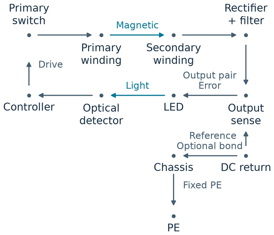
Now let the hypothetical load step up while the converter is regulating normally, with room to increase delivery. The capacitor initially makes up the shortfall and its voltage falls. In the common shunt and phototransistor arrangement considered here, the lower divider voltage makes the shunt sink less LED current. The primary receiver then conducts less, and the feedback input interprets that change as a request for more delivery. The controller can increase the energy sent per cycle, send energy more often, or use a combination, depending on its control law. As the output recovers, the sense voltage rises and the request backs off. The response has the opposite sign when the output rises above its setpoint.
The exact voltage on a controller’s feedback pin depends on the receiver circuit. For example, less phototransistor current lets a pull-up raise the pin voltage in one arrangement. A different input circuit can use another polarity. Follow what the controller does with the signal rather than assuming every falling output produces a falling feedback-pin voltage. Likewise, the direction of a correction does not tell you how fast the output settles or how far it initially drops. Those results depend on the power stage, the available control range, the output capacitor and the complete loop.
Texas Instruments’ shunt-reference note SNVAA58 and its flyback compensation report SLUA671 show how the sensing and optical stages contribute to loop behavior. The optocoupler’s current transfer ratio relates receiver current to LED current under stated conditions. A change in that ratio can change loop gain even when the output divider and voltage reference are unchanged. Bias and compensation also matter: a shunt that operates at a different current can behave differently as an error amplifier. A good nominal DC reading gives little information about those dynamic effects.
That sequence starts from normal regulation. At startup, the secondary may not yet have enough voltage to drive the LED. A weak optical signal at that point has a different meaning from a weak signal after a load step: the loop may not yet be in control. The primary controller’s startup and protection circuitry determines what switching is allowed before feedback becomes usable. The same distinction matters if the LED path opens. Loss of the signal is a feedback fault; the schematic alone does not establish whether the output overshoots, shuts down or restarts.
The divider’s location also tells you which voltage the loop will try to recover. In this example it senses at the supply output. If an industrial controller draws more current through a long pair of leads, the voltage at the controller can drop more than the voltage at the supply terminals. Even after the feedback loop restores the terminal voltage, the load can still see the drop across both conductors. Direct secondary sensing means direct observation at the chosen sense points. It does not mean the regulator sees the voltage at every load on the cable.
What the primary can infer from a flyback pulse
A flyback can use the power transformer itself to get information about the output. While the secondary rectifier is conducting, the output and rectifier path impose a voltage on the secondary winding. The turns ratio reflects that voltage onto a winding on the primary side. A controller can sample a suitably timed voltage on a primary-referenced auxiliary winding, or it can use the reflected part of the primary switch waveform. Neither approach needs a wire from the output return to the primary controller.
The distinction is visible in the examples in Analog Devices’ explanation of flyback feedback. Its traditional circuits show optical feedback and a third-winding arrangement, while its no-opto example observes the primary switch waveform. Texas Instruments’ PMP8787 reference design documents a mains-fed flyback that uses primary-side regulation without an optocoupler. These examples establish the sensing methods. The timing and circuitry in a particular supply still determine which signal it uses.
With an auxiliary winding, the useful sample comes from the interval when the secondary is delivering energy. Before scaling by the winding ratio, the relevant secondary winding voltage includes the output voltage, the forward drop of the rectifier and resistive drops associated with secondary current. Winding coupling also affects how accurately the primary-side signal represents the secondary. With switch-node sensing, the observed voltage during energy transfer includes the input bus voltage as well as the reflected contribution. The controller needs a way to distinguish the part that tracks the output.
Timing is part of the measurement. Immediately after the switch opens, leakage inductance can produce a spike and ringing. That peak is a poor stand-in for the output voltage. In a discontinuous flyback, secondary current then decays toward zero. TI’s flyback application brief SLVAFK6 explains why some controllers sample near the end of demagnetization: current-dependent drops have diminished by that point. Sampling too late can miss the useful interval, because once the rectifier stops conducting, the output no longer clamps the winding through that path. This is an example of how one sensing method works, rather than a sampling rule for every flyback.
Think through the same load step with this circuit. The primary-side controller has to wait for a usable flyback sample, then estimate whether the output moved. A different rectifier drop or a distorted sample can alter that estimate even when the actual output voltage is the same. The optical circuit starts with a direct terminal-voltage measurement, but it has its own sources of error and delay in the divider, reference, optical transfer and compensation. Neither the presence nor the absence of an optocoupler establishes which finished supply will have the smaller voltage deviation under a specified load step.
The same distinction helps explain why a light-load measurement can be revealing. If the primary controller pauses switching between bursts, there is no new flyback pulse to sample during the pause. The most recent sample describes an earlier transfer interval; it does not track the capacitor continuously. A secondary divider can still have the output across it during that pause, although its signal is useful only while the sensing and transfer circuitry remains biased. The two loops can therefore have different information available at the instant a load wakes up, before either one changes what the switch does.
This is why the two designs lead to different schematic questions. For direct secondary sensing, identify the sense points and how the error signal reaches the controller. For primary-side sensing, identify the winding or switch node and the operating interval that makes its voltage informative. A steady DC output at one load can look the same with either architecture. The circuit tells you what the controller actually observed to produce it.
An earth bond changes the reference the loop does not measure
Return to the optocoupler example. Keep protective earth (PE) connected to the enclosure in both versions. In the first version, the secondary has no deliberate conductive connection to PE or another external DC reference. The output is floating in that sense: the converter controls the voltage between its two DC terminals, while the circuit does not deliberately fix either terminal’s DC potential relative to earth. The shunt still sees its divider voltage and the primary receiver still sees light.
In the second version, assume the supply and host documentation permit a single connection from the secondary return to the enclosure’s PE node. In the simplified circuit, the bond sets the return to earth potential at the bond point. The positive terminal then sits approximately one output voltage above that point under steady conditions, with conductor drops excluded. The divider still spans the same two DC terminals. In the example, no component in the sensing or optical path moves, and PE does not take the place of the load return.
The difference can be read directly from the nodes. An output-voltage observation uses DC positive and DC return. An earth-reference observation uses one of those nodes and PE. The bond changes the second relationship while the loop continues to control the first. Moving both sense nodes together relative to earth leaves the ideal divider’s input voltage unchanged. Real equipment can have coupling and shared impedances, so this observation does not predict the effect of a bond on noise or on the voltage seen elsewhere in the installed system.
A conductive link between the primary controller’s return and the secondary return bypasses the internal isolation barrier. In the simplified cabinet drawing, the secondary bond ends at PE and there is no onward conductive path to the primary circuit. In an installed system, trace beyond the cabinet. For example, if the AC source bonds neutral to earth, the secondary return can share a conductive path with supply neutral through PE and that upstream bond. The converter’s internal insulation remains in place. The installed reference relationship depends on the complete circuit, including external interfaces.
These cases show why the DC reading can remain steady with either earth reference, even though the installed connections differ. A feedback loop can also keep regulating after an unintended conductive link joins the domains; a correct output voltage alone cannot establish isolation. They do not determine whether to bond a particular supply. For that decision, use the supply instructions and the host’s documented electrical design. Keep the required PE connection in place; the only branch varied in this comparison is the secondary reference.
Frequently Asked Questions
Does an auxiliary winding automatically mean primary-side regulation?
No. A winding on the primary side can supply bias power to the controller while an optocoupler provides the voltage feedback. Trace the winding signal to the control input and identify what sets the output voltage. Finding a bias winding alone does not identify the regulation method.
Can primary-side regulation compensate for voltage drop in the load cable?
Some controllers raise the supply-terminal voltage as output current increases to offset expected cable drop. The correction depends on how the controller is configured and on the resistance of the installed cable. The controller still estimates the correction from the supply side and has no direct measurement at the load terminals.
Does regulating one flyback output regulate every secondary winding?
Not to the same accuracy by default. If the loop senses one output, it corrects the error at that output. Additional rails can shift as their loads and rectifier drops change. An independently sensitive rail needs its own documented regulation behavior or a separate regulation stage.