A hypothetical server PSU delivers 12.08 V at 20 A and 12.00 V at 80 A after both operating points have settled. The difference is 80 millivolts. Does that establish acceptable load regulation? It establishes a voltage change between two measurements. Interpreting that change requires a fixed input condition, a defined output measurement location, and the applicable manufacturer’s regulation definition and limits.
Testing steady-state load regulation means changing permitted output demand while holding the input and other specified conditions fixed, then comparing settled voltages. This article develops that laboratory method for engineers working with a documented module and suitable fixture. Every numerical reading and acceptance window below is hypothetical. For a server that will not start or reports a PSU fault, Powernexu’s rack-side PSU troubleshooting procedure addresses the different task of locating the failed path.
Fix the output boundary and the supported operating state
Begin with the exact module identity and its applicable specification revision. The document must establish permitted input conditions, output loading, voltage limits, cooling, control states, and the manufacturer’s test method where provided. No exact-model operating specification accompanies this example, so its numbers cannot authorize testing an actual module or classify a commercial product as passing.
Choose the voltage observation location specified by that document. A measurement at the module’s defined output boundary and one at the electronic load can differ because the intervening contacts and conductors carry current. Increasing demand increases resistive distribution drop. If the voltage leads move between those locations during the sweep, the resulting difference combines changed loading with a changed measurement boundary.
The voltage instrument uses its own measurement leads connected to the fixture’s designated voltage observation points, separate from the conductors carrying the load current. Both the positive observation point and its return reference belong in the connection record. A four-wire measurement arrangement can exclude some load-lead drop, but its usefulness depends on where those separate leads actually terminate.
Instrument measurement leads and PSU remote-sense connections perform different functions. The former observe voltage; supported remote-sense connections participate in the supply’s regulation. Preserve the manufacturer’s prescribed sense arrangement throughout the comparison. Do not move sense connections to improve a reading. Powernexu’s discussion of documenting a server PSU interface explains why these assignments require exact hardware evidence.
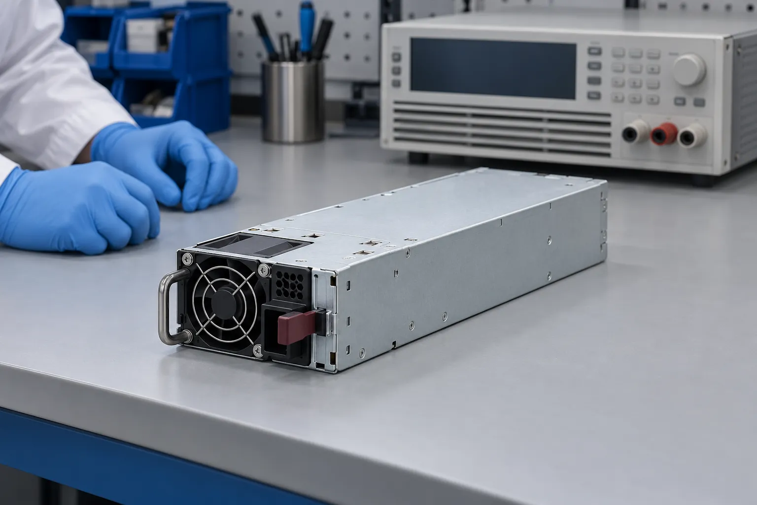
The PSU enclosure stays closed, with the documented mating assembly providing guarded electrical access. Qualified personnel should establish connections under the laboratory’s isolation procedure before energization. The fixture must preserve protective connections and the required ventilation. A generic desktop tester or an improvised jumper does not establish a supported startup arrangement for an unidentified server module.
Retain auxiliary loads, output settings, and required control connections at their specified states. If the product intentionally changes output voltage with a sharing or operating policy, that behavior belongs in the adopted interpretation. Testing a permitted standalone configuration does not automatically characterize the module while sharing current inside a server.
Separate the load sweep from the input sweep
A compact matrix can distinguish two questions. Across one row, keep input voltage fixed and change output current: this examines load-dependent variation. Down one column, keep output current fixed and change input voltage: this examines input-dependent variation. Changing both together may reveal a large difference, but it does not identify either effect separately.
Select the operating points from the exact specification and intended investigation. Include required intermediate points rather than assuming two endpoints describe the entire permitted interval. A nominal percentage of rated power is insufficient when the available output changes with input or cooling conditions. Every selected combination must remain inside the documented simultaneous operating envelope.
For the worked example, assume a fictional nominal 12 V output supports 20 A, 50 A, and 80 A at each of three AC inputs: 200 V, 230 V, and 240 V. These are stipulated permitted combinations, not recommended test settings. Assume frequency, cooling, auxiliary loading, control state, and voltage observation points remain fixed.
Use the load mode required by the adopted method. Here, constant-current operation holds each column’s demand at its stated current. Constant-power operation would alter current as output voltage changed, answering a different controlled-loading question. Record achieved current and delivered input voltage alongside their commands. A source setting alone does not establish the voltage reaching the PSU under demand.
The electronic load produces heat while absorbing PSU output. Place its exhaust so that it does not feed warmed air into the PSU inlet, and preserve the module’s specified cooling arrangement. Otherwise, later load points can acquire a different thermal condition. Physical separation and ventilation direction therefore support the assumption that the comparison holds cooling conditions fixed.
Acquire each reading after the preparation and settling required by the applicable method. There is no universal waiting period established here. If voltage continues drifting, retain that history rather than selecting a convenient instant. A return to an earlier load can reveal an order-dependent change; it does not by itself identify whether temperature or another operating condition caused it.
Calculate voltage error and regulation from the same table
The following invented readings represent settled voltage at one unchanged module-output boundary. For arithmetic only, assume an absolute output window of 11.88–12.12 V, equivalent to ±1% around the fictional 12.00 V nominal value. This window is an example requirement, not a server-PSU standard. Measurement uncertainty is omitted from the example arithmetic; a real conformity decision needs its applicable uncertainty treatment.
| Hypothetical AC input | Output at 20 A | Output at 50 A | Output at 80 A | Sampled row span |
|---|---|---|---|---|
| 200 V | 12.06 V | 12.02 V | 11.98 V | 0.08 V |
| 230 V | 12.08 V | 12.04 V | 12.00 V | 0.08 V |
| 240 V | 12.09 V | 12.05 V | 12.01 V | 0.08 V |
First compare each reading with its applicable absolute voltage limits. All nine invented central values lie inside the assumed window. That observation does not require a regulation calculation. It answers whether the sampled voltages satisfy the stipulated absolute bounds under direct numerical comparison, leaving measurement uncertainty outside this simplified finding.
Next calculate signed endpoint change at one fixed input. At 230 V AC, subtract the 20 A reading from the 80 A reading: 12.00 V − 12.08 V = −0.08 V. The negative sign describes a reduction as current increases. Keeping that sign preserves information that disappears when reporting only a positive percentage.
For this example, define normalized endpoint change using nominal output voltage as the denominator: 100 × (−0.08 V) ÷ 12.00 V = approximately −0.667%. State the denominator explicitly. Dividing by the initial measured voltage would produce a different number. Use the manufacturer’s convention when assessing its published regulation claim rather than silently substituting this example definition.
A sampled maximum-to-minimum span answers another question. At 230 V, the highest listed voltage is 12.08 V and the lowest is 12.00 V. Their span is 0.08 V, or approximately 0.667% of nominal. These endpoints happen to contain the extrema in this row. That coincidence should not become an assumption for subsequent measurements.
Absolute nominal error remains separate. The table’s highest reading, 12.09 V, is 0.09 V above nominal, corresponding to +0.75%. Its lowest reading, 11.98 V, is approximately 0.167% below nominal. Neither figure equals the fixed-input load span. A supply can have a small load-dependent change while its entire output range sits too high or too low.
Laboratory equipment supports these controlled comparisons. Keysight’s server PSU validation overview identifies electronic loads and automation among the testing tools. Such equipment provides controllable demand and repeatable acquisition; it does not supply the missing acceptance limits for an unidentified module. Those remain attached to the adopted product specification.
A small endpoint difference can hide an intermediate failure
Now change one hypothetical value: replace the 230 V, 50 A reading with 12.14 V. Keep the 20 A and 80 A readings unchanged. The endpoint difference remains −0.08 V, and the endpoint calculation still returns approximately −0.667%. An endpoint-only report would conceal the changed middle of the row.
The altered intermediate reading exceeds the assumed 12.12 V upper bound by 0.02 V. The sampled maximum-to-minimum span also changes: 12.14 V − 12.00 V = 0.14 V, approximately 1.167% of nominal. The absolute-limit comparison and the span calculation now expose information that the unchanged endpoint statistic misses.
This example illustrates why the required point coverage belongs in the method. It does not imply that an arbitrary three-point sweep proves acceptable voltage everywhere between its samples. Additional points may be required by the manufacturer’s procedure or justified by observed behavior. A narrow feature between sampled currents can remain undiscovered even when every listed value is acceptable.
In a real measurement, proximity to a limit also raises the decision-rule question. Display resolution, calibration, connection effects, repeatability, and the relevant uncertainty evaluation affect what the evidence can distinguish. Do not round a reading toward the acceptable side before comparison. Retain sufficient digits for evaluation and report the resulting precision honestly.
If a point appears outside its limit, preserve its conditions and acquisition record before changing settings. Averaging it together with acceptable points answers no useful absolute-limit question. Likewise, adjusting the output setpoint separately at each current would remove the very variation the load sweep was intended to measure.
Repeat the load comparison at each input condition
Return to the original table. At 20 A, changing input from 200 V to 240 V changes output from 12.06 V to 12.09 V. The sampled input-dependent span is 0.03 V, or 0.25% of nominal. The other two current columns have the same span in this invented dataset; actual products need not preserve that pattern.
Compare this with the 0.08 V load span within each input row. The two statistics describe different controlled changes. Selecting the highest table value, 12.09 V, and subtracting the lowest, 11.98 V, gives 0.11 V across the sampled matrix. That combined span is useful when explicitly named, but calling it load regulation would hide the simultaneous input change.
Input-dependent capacity can restrict the matrix itself. If an actual specification permits less current at one input, a high-current cell outside that envelope should be excluded or replaced with an authorized point. Its absence is meaningful coverage information. It cannot be filled by extrapolating a favorable reading from a higher-input row.
The original example therefore supports three numerical descriptions: a sampled 0.08 V load span at each stated input, a sampled 0.03 V input-dependent span at each stated current, and nine central readings inside the invented absolute window. No separate percentage regulation acceptance threshold was stipulated, so the span calculation cannot establish compliance with one.
Those settled readings leave the intervening load transitions uncharacterized. Startup, ripple, rapid voltage excursions, and recovery require their own observation methods and limits. Similarly, a matrix taken at one cooling condition supplies no measurements at another. The useful result is the actual voltage surface sampled under the declared conditions, with its absolute-limit comparisons and calculation conventions preserved.