Two conducted EMI plots can disagree even when the industrial power supply has not changed. A different load, measurement network, detector, or output-cable arrangement can change what reaches the receiver. Conducted EMI testing for industrial power supplies becomes useful when those conditions are documented well enough to reproduce the result and distinguish an electrical change from a measurement change.
For mains-port precompliance work, the immediate objective is to measure radio-frequency disturbance leaving the equipment through its supply connection under defined operating conditions. A line impedance stabilization network, or LISN, provides the specified measurement interface. The resulting spectrum helps locate problems and compare revisions; a bench trace alone does not establish conformity of the finished machine. Start by deciding which port, equipment configuration, and operating state the trace represents.
Define the observation before selecting a limit line
An industrial supply may be examined as a component on a controlled fixture or inside the equipment it powers. Those observations answer different questions. The component arrangement can support comparisons between samples or design revisions. The assembled-equipment arrangement includes the controller, DC harness, enclosure, and other active circuits that may contribute noise or provide coupling paths.

Name that boundary in the test record. “AC input of the assembled inspection controller” is more informative than “PSU EMI.” Identify whether the receiver is observing an individual input conductor, which other conductors are present, and how auxiliary ports are configured. A plot from one measured line should not silently stand for every required line or port.
The applicable requirement follows the equipment and intended application. Texas Instruments’ overview of conducted EMI specifications illustrates why different product sectors use different emissions requirements and detector criteria. It is a historical engineering overview, not a substitute for the applicable standard and edition. Obtain the actual method, classification, frequency coverage, and limits for the intended assessment before attaching a compliance label to a trace.
Conducted emissions also differ from conducted immunity. Emissions testing observes disturbance produced by operating equipment. Immunity testing applies a defined disturbance and observes equipment behavior. A controller that operates normally during an emissions sweep has not thereby passed an immunity test; a successful immunity exposure does not establish low emissions.
The LISN and receiver form a measurement chain
The LISN helps establish a defined radio-frequency impedance at the equipment’s power port and couples disturbance to the measuring instrument. Its type and usable frequency range belong in the configuration. An arbitrary network selected because its connectors fit may produce a repeatable-looking result that is not comparable with the intended method.
Specify the network model, calibration status, measured port, and the treatment of unused measurement ports according to the network instructions and test method. Record the receiver or analyzer, RF cable, limiter, attenuation, and any preamplifier. Together these determine the usable signal range and the corrections needed to refer the displayed voltage to the observation point.
A pulse limiter protects an instrument within its documented capabilities; it does not make every connection safe or every transient harmless. Mains LISNs require the laboratory’s approved protective-earth arrangement, rated equipment, and operating procedure. Qualified personnel should establish that arrangement from the equipment instructions. Lifting protective earth to obtain a quieter trace changes the electrical system and can create a hazardous condition.
Check the measurement chain before diagnosing the converter. Excessive attenuation can bury a small signal in the noise floor. Insufficient input protection or headroom can overload the receiver. An overloaded input may produce misleading spectral content, so a crowded display is not sufficient evidence that every visible peak originates in the supply.
Document whether stored traces already include cable loss, network correction, and limiter insertion loss. Apply each correction once. If software exports both raw and corrected values, label them explicitly; otherwise a later spreadsheet can add an existing correction again and manufacture a change that never occurred electrically.
Peak, quasi-peak, and average traces answer different questions
A detector describes how the instrument turns the signal passing through its measurement bandwidth into a reported level. Peak detection captures high excursions. Quasi-peak detection weights repetitive disturbances through a defined response. Average detection reports a different weighted measure of the signal. Their readings depend on the disturbance’s time behavior as well as its amplitude.
A fast peak prescan is useful for finding candidate frequencies and operating states. It does not justify calling a peak crossing of a quasi-peak limit a confirmed quasi-peak failure. Investigate the candidate using the specified detector and measurement timing. Conversely, a rushed sweep can miss intermittent activity and should not support a confident pass merely because its displayed line is low.
Resolution bandwidth, frequency step, dwell time, sweep behavior, and detector selection must accompany the result. Narrowing a bandwidth can change the displayed level, especially for broadband or modulated noise. Changing settings between two engineering revisions undermines the comparison unless the effect is understood and the relevant measurements are repeated consistently.
Intermittent operating states need observation time that actually includes them. An industrial controller may transmit data periodically or enable a peripheral only during a production cycle. A sweep performed while that peripheral is idle can describe idle emissions accurately while missing the condition the engineer intended to investigate. Relate the acquisition to the operating sequence rather than assuming one sweep sees everything.
Keep detector identity attached to every marker value. A report that lists a frequency and a voltage without detector and bandwidth invites a false comparison. Where the applicable method requires more than one detector criterion, assess each required result against its corresponding limit, rather than choosing whichever trace looks most favorable.
The load and DC harness are part of the experiment
A resistive load offers a controlled way to compare the supply at defined output currents. An electronic load can provide flexible settings, but its own switching, control loop, chassis connections, and attached monitoring equipment may affect the observation. The actual controller introduces another set of operating states. Equal average output power does not make these loads electromagnetically equivalent.
MEAN WELL’s component-power-supply test statement describes representative arrangements with specified load conditions and output-wire placement, including application-specific loads where appropriate. The useful lesson is to obtain the manufacturer’s actual test arrangement before comparing its component result with an assembled machine. Copying a load percentage while changing the physical return paths does not recreate that arrangement.
Record the load model and mode, current setting, measured output voltage, and connections to other equipment. Note whether communications, remote sense, or monitoring cables are attached. An oscilloscope or laptop added for convenience can create another coupling route. Removing that accessory later may alter the result even though the PSU and programmed load remain unchanged.
Output-harness length, routing, separation, shielding, and intentional connections to chassis must be reproducible. Photograph the whole fixture and preserve the relevant dimensions in a drawing. A photograph alone can hide cable height or a bond underneath the mounting plate; a written description alone may miss an unintended cable loop.
Include intended light-load and active-load states where relevant to the product. Some converters change operating mode as demand falls, so full output is not automatically the loudest condition at every frequency. Record input voltage and frequency, warm-up condition, and enabled auxiliaries. Choose the operating matrix from the intended use and the applicable method rather than treating a single convenient point as representative.
Separate background, fixture effects, and equipment noise
Before interpreting a troublesome frequency, establish what the measurement environment contributes. A background observation made with the equipment under test inactive, using the laboratory’s safe procedure, can reveal persistent external signals or instrument artifacts. Preserve the exact background configuration: turning equipment off can also change terminations and coupling, so background subtraction is not automatically valid.
If a feature appears in both background and powered observations, mark it for investigation rather than deleting it. If a feature appears only during operation, correlate it with operating state. A repeated pattern of peaks may suggest switching-related activity, but appearance alone does not identify a specific internal component or distinguish common-mode from differential-mode noise.
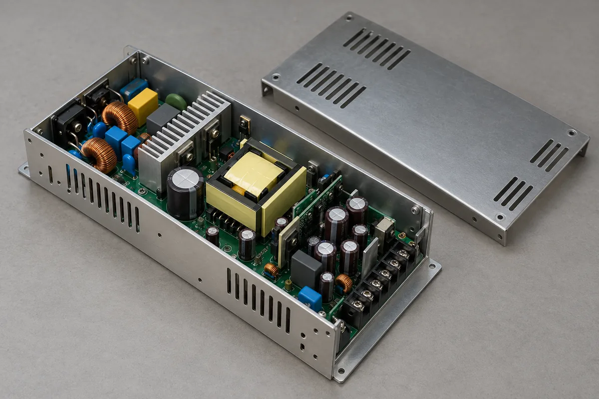
Mode separation requires an appropriate diagnostic method and a suitable measurement arrangement. A single LISN voltage trace does not independently identify the noise mode. Choosing a common-mode choke simply because a peak sits at a particular frequency can waste time when the dominant path has not been established.
Make a deliberate diagnostic change and preserve the original baseline. For example, compare the actual controller with a controlled resistive load while holding the intended supply operating point and fixture geometry as closely as practical. A changed spectrum directs attention toward load behavior or associated coupling; it does not prove the controller is defective. The load substitution itself changes the experiment.
After the diagnostic observation, restore the baseline and repeat it. If the original trace does not return within the observed repeatability, investigate drift, operating-state changes, or disturbed connections before crediting the modification. This return measurement prevents an accidental fixture movement from being recorded as a successful filter improvement.
Reconcile two traces before redesigning the filter
Consider a hypothetical review in which a supplier’s component plot looks lower than the machine integrator’s bench result. The supplier used a resistive load and a defined output harness. The integrator used the production controller, an attached programming laptop, and a different receiver setup. Neither plot needs to be fraudulent for the comparison to be invalid.
First align the observed port, detector, bandwidth, and correction basis. If one marker is corrected quasi-peak and the other is an uncorrected peak value, the difference is not yet a measured degradation of the machine. Keep both original records, then obtain a comparable acquisition. Do not apply an assumed offset between detectors; the relationship depends on signal behavior.
Next separate the configuration questions. Reproducing the documented component fixture can test whether the integrator obtains a broadly consistent component observation. Measuring the production assembly answers what the intended equipment emits. A good match in the first arrangement does not erase a problem in the second, but it narrows the investigation away from a simple sample discrepancy.
A comparison log should connect each trace to a configuration revision and describe exactly what changed. Store native data and instrument settings alongside the plot image. Include the frequencies under investigation, measured line, detector, operating state, and whether the values are corrected. This lets another engineer revisit the observation without reverse-engineering a screenshot.
When reporting margin, use the applicable limit minus the corrected measurement for the same frequency and detector. An internal target can allow room for repeatability, sample variation, and later integration changes, but it should be identified as an engineering target rather than an invented regulatory requirement. The laboratory’s formal assessment must use its applicable method and uncertainty treatment.
The useful outcome of this hypothetical comparison might be that the component result is reproducible, while connecting the production controller introduces a repeatable increase in a particular band. That statement supports a focused investigation of the assembled load and coupling paths. It is more actionable than declaring the supply “bad,” and more honest than treating an attractive component plot as the finished machine’s result.